pytrick or gist

区分一维数组和 行变量 列变量

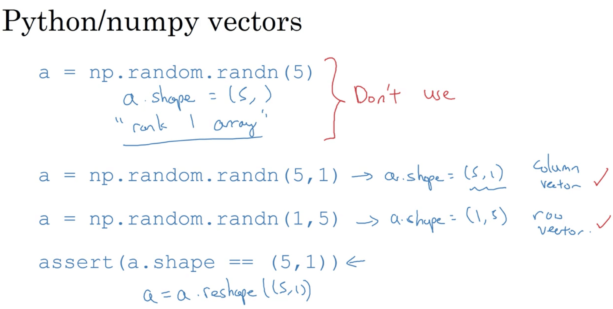
一维数组 行为 不总与行变量or列变量一直,造成不必要的bug。总是使用nx1维矩阵(基本上是列向量), 或者1xn维矩阵(基本上是行向量),这样你可以减少很多assert语句来节省核矩阵和数组的维数的时间。 另外,为了确保你的矩阵或向量所需要的维数时,不要羞于reshape操作。

1
2
3
4
5
6
7
8
9
10
11
12
np.random.randint(5)
a = np.random.randn(5)
>>> array([-1.05118915, -0.45812568,  0.28528316,  0.75364257,  1.23234449])
>>> a.shape
(5,)


b = a.reshape(1,-1)
>>> array([[-1.05118915, -0.45812568,  0.28528316,  0.75364257,  1.23234449]])
>>> b.shape
(1, 5)

sklearn

train_test_split

1
2
3
4
5
6
7
8
9
import numpy as np

def split_train_test(data, test_ratio):
    shuffled_indices = np.random.permutation(len(data))
    test_set_size = int(len(data) * test_ratio)
    test_indices = shuffled_indices[:test_set_size]
    train_indices = shuffled_indices[test_set_size:]
    return data.iloc[train_indices], data.iloc[test_indices]

sklearn

1
2
3
4

from sklearn.model_selection import train_test_split
train_set, test_set = train_test_split(housing, test_size=0.2, random_state=42)

clean

处理文本和类别属性 文本标签转换为数字

1
2
3
4
5
6
7
8
9
10
11
12
13
14
15
16
17
18
# 这种做法的问题是,ML 算法会认为两个临近的值比两个疏远的值要更相似
from sklearn.preprocessing import LabelEncoder
encoder = LabelEncoder()
housing_cat = housing["ocean_proximity"]
housing_cat_encoded = encoder.fit_transform(housing_cat)
>>> print(encoder.classes_)
['<1H OCEAN' 'INLAND' 'ISLAND' 'NEAR BAY' 'NEAR OCEAN']

# 常见的方法是给每个分类创建一个二元属性 独热编码(One-Hot Encoding),因为只有一个属性会等于 1(热),其余会是 0(冷)

"""
注意输出结果是一个 SciPy 稀疏矩阵,而不是 NumPy 数组。当类别属性有数千个分类时,这样非常有用。
经过独热编码,我们得到了一个有数千列的矩阵,这个矩阵每行只有一个 1,其余都是 0。
使用大量内存来存储这些 0 非常浪费,所以稀疏矩阵只存储非零元素的位置。
"""
from sklearn.preprocessing import OneHotEncoder
encoder = OneHotEncoder()
housing_cat_1hot = encoder.fit_transform(housing_cat_encoded.reshape(-1,1))

使用类LabelBinarizer,我们可以用一步执行这两个转换(从文本分类到整数分类LabelEncoder,再从整数分类到独热向量OneHotEncoder

1
2
3
4
5
6
7
8
9
10
11
>>> from sklearn.preprocessing import LabelBinarizer
>>> encoder = LabelBinarizer()
>>> housing_cat_1hot = encoder.fit_transform(housing_cat)
>>> housing_cat_1hot
array([[0, 1, 0, 0, 0],
       [0, 1, 0, 0, 0],
       [0, 0, 0, 0, 1],
       ...,
       [0, 1, 0, 0, 0],
       [1, 0, 0, 0, 0],
       [0, 0, 0, 1, 0]])
1
2
3
4
5
6
7
pandas
>>> labels, uniques = pd.factorize(['b', 'b', 'a', 'c', 'b'])
>>> labels
array([0, 0, 1, 2, 0])
>>> uniques
array(['b', 'a', 'c'], dtype=object)

Pipeline

Sequentially apply a list of transforms and a final estimator. Intermediate steps of the pipeline must be ‘transforms’, that is, they must implement fit and transform methods. The final estimator only needs to implement fit.

当你调用流水线的fit()方法,就会对所有转换器顺序调用fit_transform()方法, 将每次调用的输出作为参数传递给下一个调用,一直到最后一个估计器,它只执行fit()方法。

1
2
3
4
5
6
7
8
9
10
11
from sklearn.pipeline import Pipeline
from sklearn.preprocessing import StandardScaler

num_pipeline = Pipeline([
        ('imputer', Imputer(strategy="median")),
        ('attribs_adder', CombinedAttributesAdder()),
        ('std_scaler', StandardScaler()),
        ])

housing_num_tr = num_pipeline.fit_transform(housing_num)

Pipeline 合并 并行执行,等待输出,然后将输出合并起来,并返回结果

1
2
3
4
5
6
7
8
9
10
11
12
13
14
15
16
17
18
19
20
21
from sklearn.pipeline import FeatureUnion

num_attribs = list(housing_num)
cat_attribs = ["ocean_proximity"]

num_pipeline = Pipeline([
        ('selector', DataFrameSelector(num_attribs)),
        ('imputer', Imputer(strategy="median")),
        ('attribs_adder', CombinedAttributesAdder()),
        ('std_scaler', StandardScaler()),
    ])

cat_pipeline = Pipeline([
        ('selector', DataFrameSelector(cat_attribs)),
        ('label_binarizer', LabelBinarizer()),
    ])

full_pipeline = FeatureUnion(transformer_list=[
        ("num_pipeline", num_pipeline),
        ("cat_pipeline", cat_pipeline),
    ])

评估

1
2
3
4
5
6
7
8
9
10
11
12
13
14
15
16
17
18
19
20
21
22
23
24
25
26
27
28
29
# mse rmse
from sklearn.metrics import mean_squared_error
mse = mean_squared_error(y_true, y_pred)
rmse = np.sqrt(mse)

# 混淆矩阵
from sklearn.model_selection import cross_val_predict
y_train_pred = cross_val_predict(sgd_clf, X_train, y_train_5, cv=3)

from sklearn.metrics import confusion_matrix
confusion_matrix(y_train_5, y_train_pred)
array([[53272, 1307],
        [ 1077, 4344]])
tn,fp
fn,tp


# 准确率与召回率
>>> from sklearn.metrics import precision_score, recall_score
>>> precision_score(y_train_5, y_pred) # == 4344 / (4344 + 1307)
0.76871350203503808
>>> recall_score(y_train_5, y_train_pred) # == 4344 / (4344 + 1077)
0.79136690647482011


# F1 值
>>> from sklearn.metrics import f1_score
>>> f1_score(y_train_5, y_pred)
0.78468208092485547

决策分数 阈值

1
2
3
4
5
6
7
8
9
10
11
12
13
14
15
16
17
18
19
>>> y_scores = sgd_clf.decision_function([some_digit])
>>> y_scores
array([ 161855.74572176])
>>> threshold = 0
>>> y_some_digit_pred = (y_scores > threshold)
array([ True], dtype=bool)

画图
from sklearn.metrics import precision_recall_curve
precisions, recalls, thresholds = precision_recall_curve(y_train_5, y_scores)

def plot_precision_recall_vs_threshold(precisions, recalls, thresholds):
    plt.plot(thresholds, precisions[:-1], "b--", label="Precision")
    plt.plot(thresholds, recalls[:-1], "g-", label="Recall")
    plt.xlabel("Threshold")
    plt.legend(loc="upper left")
    plt.ylim([0, 1])
plot_precision_recall_vs_threshold(precisions, recalls, thresholds)
plt.show()

save/load

1
2
3
from sklearn.externals import joblib
joblib.dump(my_model, "my_model.pkl")
my_model_loaded = joblib.load("my_model.pkl")

交叉验证

1
2
3
4
5
from sklearn.model_selection import cross_val_score
# K-fold cross-validation
scores = cross_val_score(reg, X, y,scoring="neg_mean_squared_error", cv=10)
rmse_scores = np.sqrt(-scores)

超参数微调

GridSearchCV

1
2
3
4
5
6
7
8
9
10
11
12
13
from sklearn.model_selection import GridSearchCV

param_grid = [
    {'n_estimators': [3, 10, 30], 'max_features': [2, 4, 6, 8]},
    {'bootstrap': [False], 'n_estimators': [3, 10], 'max_features': [2, 3, 4]},
  ]

forest_reg = RandomForestRegressor()

grid_search = GridSearchCV(forest_reg, param_grid, cv=5,
                           scoring='neg_mean_squared_error')

grid_search.fit(housing_prepared, housing_labels)

网格搜索会探索12 + 6 = 18种RandomForestRegressor的超参数组合,会训练每个模型五次(因为用的是五折交叉验证)。 换句话说,训练总共有18 × 5 = 90轮!K 折将要花费大量时间,完成后,你就能获得参数的最佳组合.

1
2
3
4
5
6
7
8
9
10
11
12
13
14
15
16
17
18
19
20
21
22
23
>>> grid_search.best_params_
{'max_features': 6, 'n_estimators': 30}
>>> grid_search.best_estimator_
RandomForestRegressor(bootstrap=True, criterion='mse', max_depth=None,
           max_features=6, max_leaf_nodes=None, min_samples_leaf=1,
           min_samples_split=2, min_weight_fraction_leaf=0.0,
           n_estimators=30, n_jobs=1, oob_score=False, random_state=None,
           verbose=0, warm_start=False)

>>> cvres = grid_search.cv_results_
... for mean_score, params in zip(cvres["mean_test_score"], cvres["params"]):
...     print(np.sqrt(-mean_score), params)
...
52172.0292957 {'max_features': 6, 'n_estimators': 10}
49958.9555932 {'max_features': 6, 'n_estimators': 30}
59122.260006 {'max_features': 8, 'n_estimators': 3}
52441.5896087 {'max_features': 8, 'n_estimators': 10}
50041.4899416 {'max_features': 8, 'n_estimators': 30}
62371.1221202 {'bootstrap': False, 'max_features': 2, 'n_estimators': 3}
54572.2557534 {'bootstrap': False, 'max_features': 2, 'n_estimators': 10}
59634.0533132 {'bootstrap': False, 'max_features': 3, 'n_estimators': 3}
52456.0883904 {'bootstrap': False, 'max_features': 3, 'n_estimators': 10}

随机搜索

当超参数的搜索空间很大时,最好使用RandomizedSearchCV

通过选择每个超参数的一个随机值的特定数量的随机组合。这个方法有两个优点:

  • 如果你让随机搜索运行,比如 1000 次,它会探索每个超参数的 1000 个不同的值(而不是像网格搜索那样,只搜索每个超参数的几个值)。
  • 你可以方便地通过设定搜索次数,控制超参数搜索的计算量。

feature select

1
2
3
4
5
6
7
8
9
10
11
12
13
14
15
16
17
18
feature_importances = grid_search.best_estimator_.feature_importances_
>>> sorted(zip(feature_importances,attributes), reverse=True)
[(0.32649798665134971, 'median_income'),
 (0.15334491760305854, 'INLAND'),
 (0.11305529021187399, 'pop_per_hhold'),
 (0.07793247662544775, 'bedrooms_per_room'),
 (0.071415642259275158, 'longitude'),
 (0.067613918945568688, 'latitude'),
 (0.060436577499703222, 'rooms_per_hhold'),
 (0.04442608939578685, 'housing_median_age'),
 (0.018240254462909437, 'population'),
 (0.01663085833886218, 'total_rooms'),
 (0.016607686091288865, 'total_bedrooms'),
 (0.016345876147580776, 'households'),
 (0.011216644219017424, '<1H OCEAN'),
 (0.0034668118081117387, 'NEAR OCEAN'),
 (0.0026848388432755429, 'NEAR BAY'),
 (8.4130896890070617e-05, 'ISLAND')]

学习曲线

1
2
3
4
5
6
7
8
9
10
11
12
13
14
from sklearn.metrics import mean_squared_error
from sklearn.model_selection import train_test_split

def plot_learning_curves(model, X, y):
    X_train, X_val, y_train, y_val = train_test_split(X, y, test_size=0.2)
    train_errors, val_errors = [], []
    for m in range(1, len(X_train)):
        model.fit(X_train[:m], y_train[:m])
        y_train_predict = model.predict(X_train[:m])
        y_val_predict = model.predict(X_val)
        train_errors.append(mean_squared_error(y_train_predict, y_train[:m]))
        val_errors.append(mean_squared_error(y_val_predict, y_val))
plt.plot(np.sqrt(train_errors), "r-+", linewidth=2, label="train")
plt.plot(np.sqrt(val_errors), "b-", linewidth=3, label="val")

pandas

summary

pd compare sql pd index slice etc

plot

1
housing.plot(kind="scatter", x="median_income",y="median_house_value",alpha=0.1)

关系

1
2
3
4
5
corr_matrix = housing.corr()

corr_matrix["median_house_value"].sort_values(ascending=False)

pd.value_counts() .info() scatter_plot .head() .describe()

数据清洗

用DataFrame的dropna(),drop(),和fillna()方法,可以方便地实现

1
2
3
4
housing.dropna(subset=["total_bedrooms"])    # 选项1
housing.drop("total_bedrooms", axis=1)       # 选项2
median = housing["total_bedrooms"].median()
housing["total_bedrooms"].fillna(median)     # 选项3

scipy

1
2
scipy.misc.imread(img_name)
scipy.misc.imresize(, (32, 32))

应用

1
2
3
4
5
6
7
8
9
10
11
12
13
14
15
df = pd.DataFrame(depth, columns=['price', 'amount'])
if not is_bids:
    # asks 保留grad位+1
    df['price'] = df['price'].apply(lambda x: math.ceil(x / g) * g)
df['price'] = df['price'].apply(cut, grad=grad)
ts = df.groupby('price', sort=False).agg({
    'amount': 'sum',
})
# if is_bids:
#     ts.sort_index(ascending=False, inplace=True)
# else:
#     ts.sort_index(inplace=True)
ts.reset_index(inplace=True)
ts['amount'] = np.round(ts['amount'], 8)
depth_list = ts.values.tolist()
1
2
3
4
5
6
7
8
9
10
11
12
13
14
15
16
17
18
19
20
21
22
23
df = pd.DataFrame(data).set_index("date")
df["price"] = df["price"].astype("float64")
all_list = filter(lambda x: x < self.support_min_period, const.MINUTE.ALL)
for m in all_list:
    self.bar_table_name = self.table_name_format % m
    resample_data = df.resample(const.PDMINUTE.NAME_DICT[m]).apply({"price": "ohlc", "amount": "sum"})

    # ohlc fillna
    resample_data.columns = resample_data.columns.droplevel()
    resample_data["date"] = resample_data.index
    resample_data['timestamp'] = resample_data['date'].apply(util.dt2ts)
    resample_data['status'] = const.KLINE_STATUS.TRADE
    resample_data = resample_data.apply(
        lambda x: x.fillna(resample_data['close'].fillna(method='ffill'))
    )
    # sum fill0
    resample_data.rename(columns={"amount": "volume"}, inplace=True)
    # resample_data["volume"] = resample_data['volume'].replace(to_replace=0, method="ffill")
    #
    resample_data = self._poloniex_5_1(m, resample_data)

    rows = resample_data.to_dict('records')

1
2
3
4
5
df['timestamp'] = df['date'].apply(cls.dt2ms)
df['timestamp'] = df['timestamp'].astype('int64')
df.drop('date', axis=1, inplace=True)
df.sort_values('timestamp', inplace=True)
rows = df[['timestamp', 'open', 'high', 'low', 'close', 'volume']].values.tolist()
1
2
3
4
5
6
7
8
9
10
df = pd.DataFrame(data).sort_values(by="date").set_index("date")
# ohlc fillna
resample_data["date"] = resample_data.index
resample_data['timestamp'] = resample_data['date'].apply(util.dt2ts)
resample_data['status'] = const.KLINE_STATUS.MERGE
close = resample_data['close'].fillna(method='ffill')
resample_data = resample_data.apply(lambda x: x.fillna(close))
# sum fill0
# resample_data["volume"] = resample_data['volume'].replace(to_replace=0, method="ffill")
rows = resample_data.to_dict('records')