小知识
一个BGR图像 0~255
ROI
更改图像的特定区域 Region Of Interest ROI 感兴趣区域
mask 掩膜
0 黑 255 白
与目标图像做mask操作 目标图像扣走mask中黑色轮廓部分,保留白色区域 => 保留ROI,其他区域为0
通常mask之前
- 先转成灰度图像
- 二值化、反二值化
作用
- 对自己做mask 可以抠图
- 提取ROI
- 特征提取
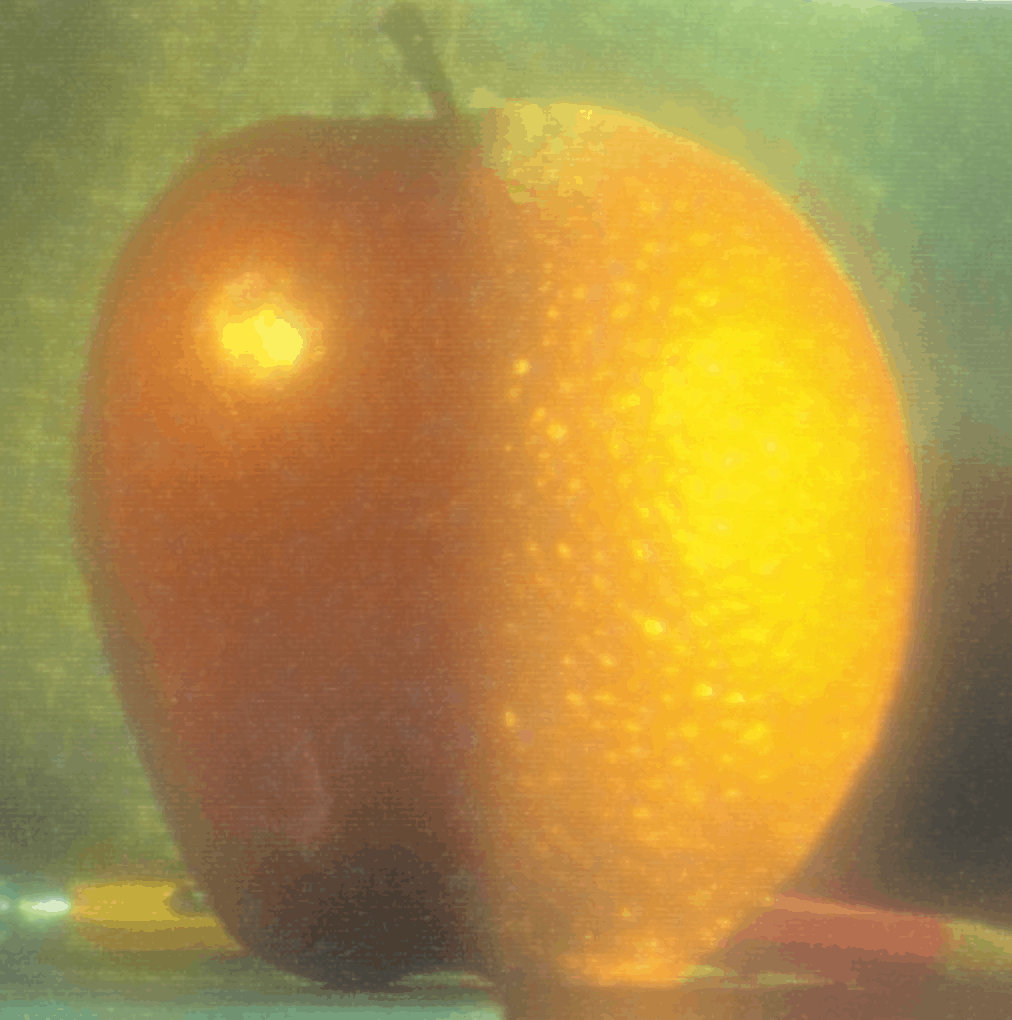
hsv
BGR和HSV的转换使用 cv.COLOR_BGR2HSV
- H表示色彩/色度,取值范围 [0,179]
- S表示饱和度,取值范围 [0,255]
- V表示亮度,取值范围 [0,255]
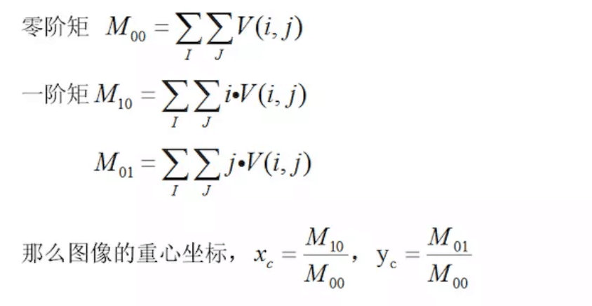
图像矩
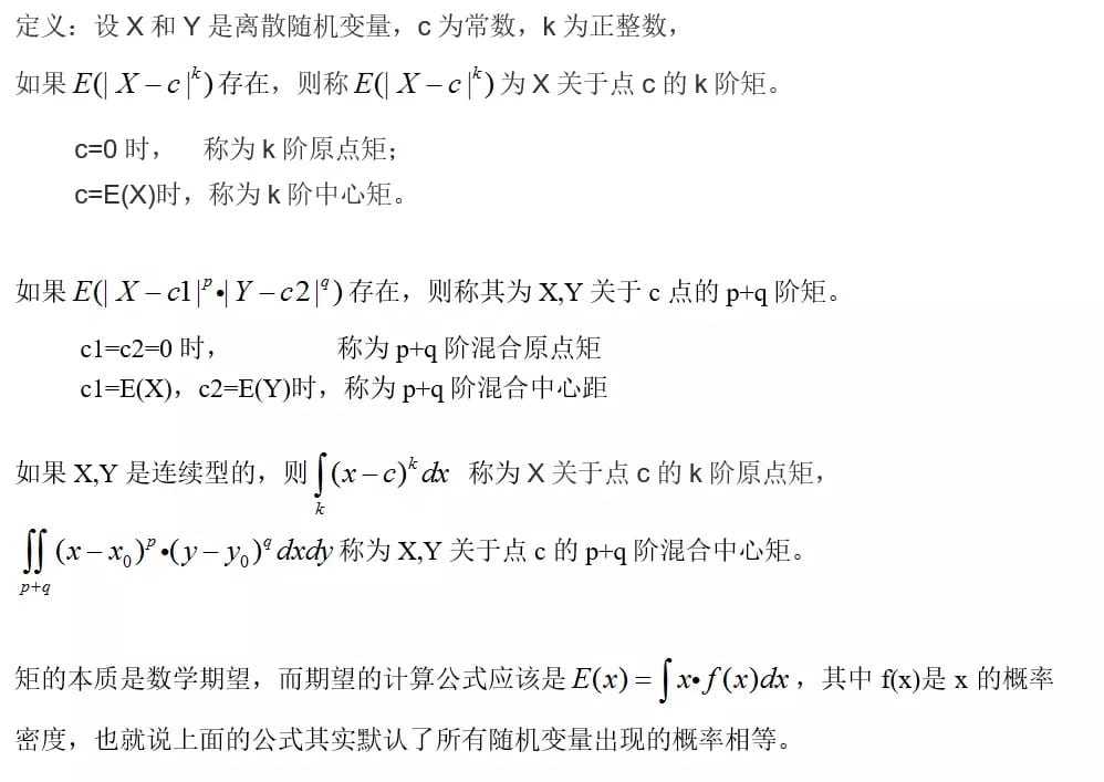
图像矩一般都是原点矩
- 一阶矩和零阶矩,计算形状的质心
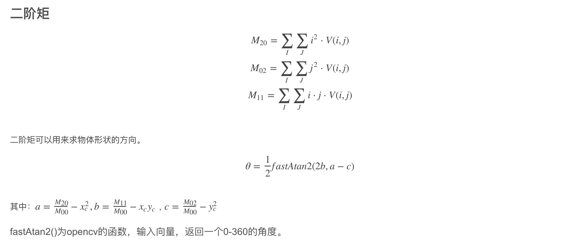
- 二阶矩,计算形状的方向
V(i,j)表示图像在(i,j)点上的灰度值。
二阶矩,计算形状的方向
基本
read write show
获取图片 路径不对,imread get None
1 | |
属性
1 | |
选取 ROI
选取区域
1 | |
单个选取
1 | |
split merge
1 | |
运算
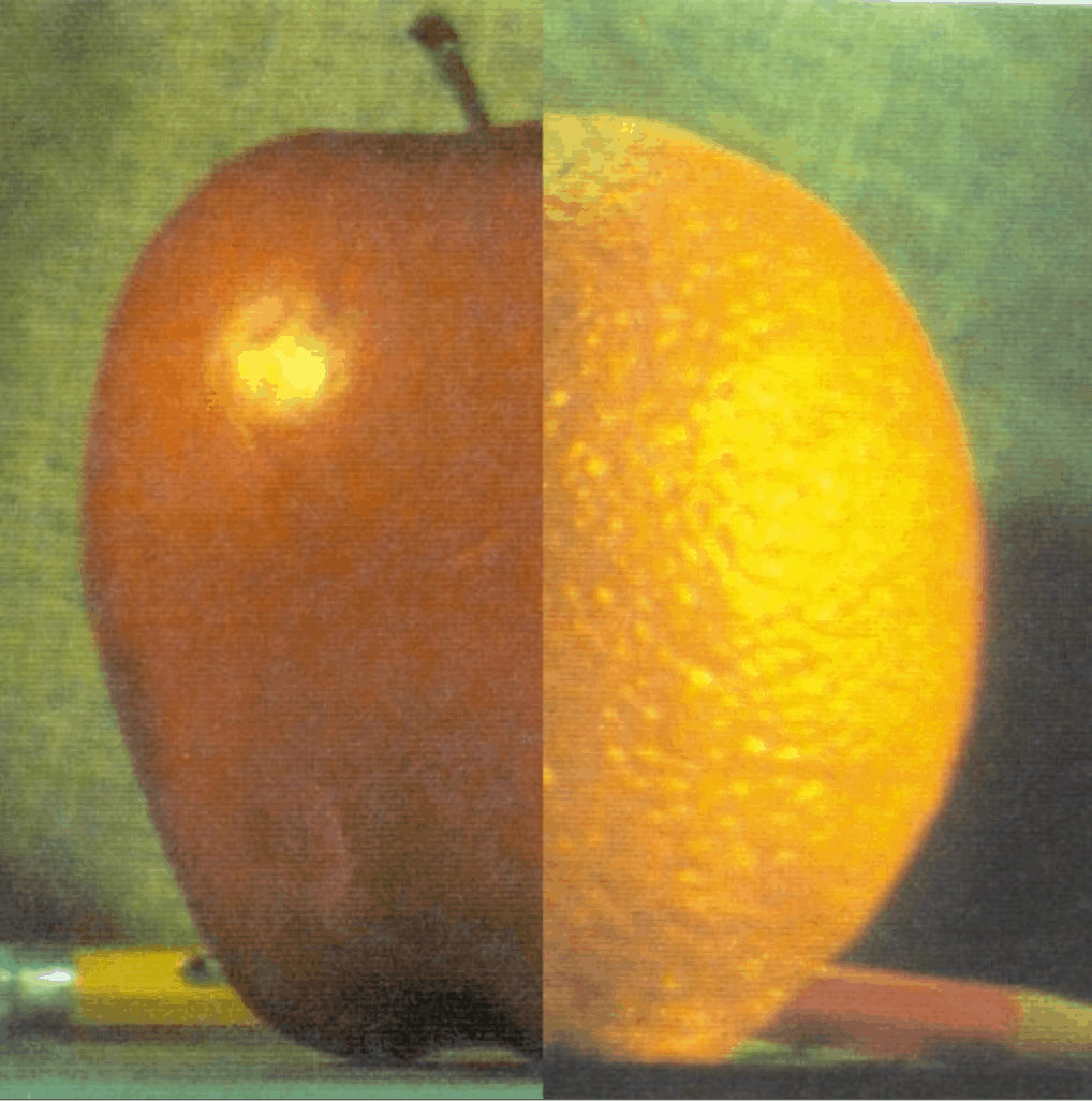
add addWeighted
Both images should be of same depth and type, (shape and 图片后缀)or second image can just be a scalar value.
1 | |
位运算
1 | |
color
灰度
1 | |
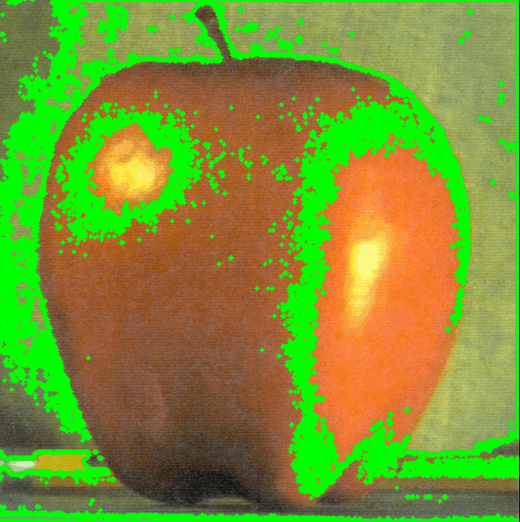
HSV
选取颜色ROI视频
1 | |
几何变换
放大缩小
1 | |
平移
1 | |
旋转
1 | |
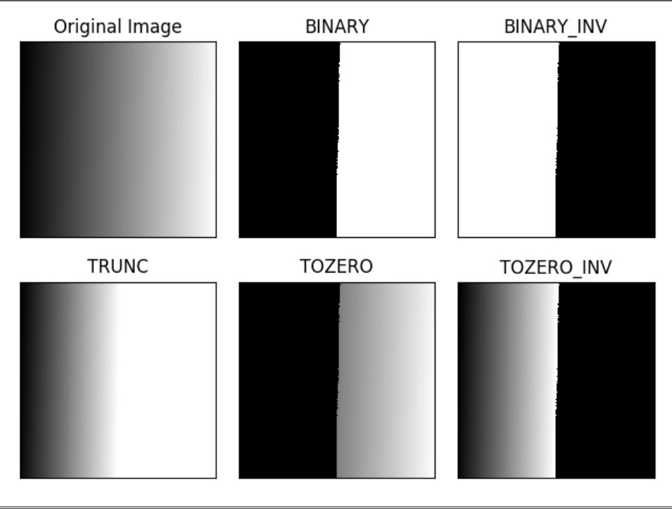
二值化 threshold
自定义全局值
1 | |
自适应阈值
1 | |

OTSU
适合双峰图
1 | |
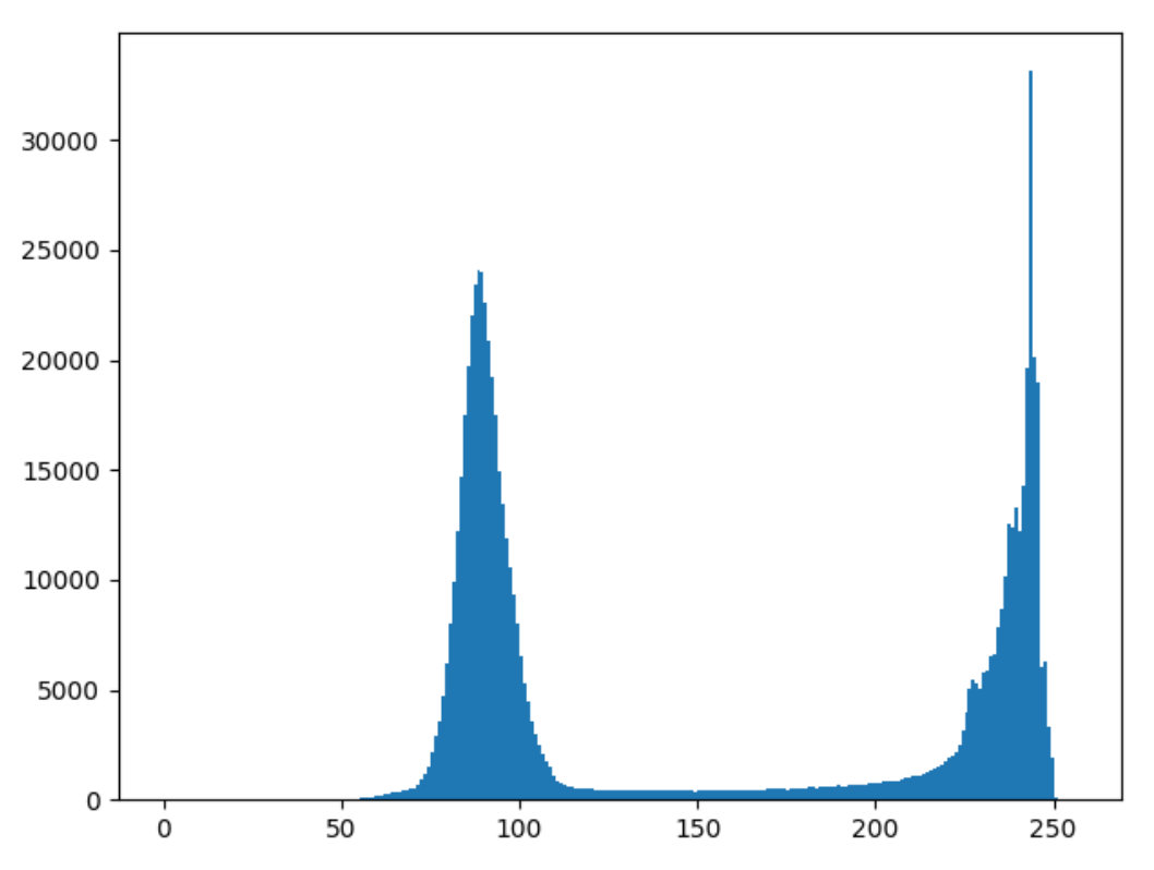
cv.THRESH_OTSU效果更好
1 | |
过滤 smooth 消除噪音
1 | |
morphological 侵蚀和膨胀
形态学运算符是 侵蚀和膨胀
1 | |
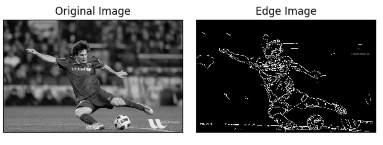
边界识别
1 | |
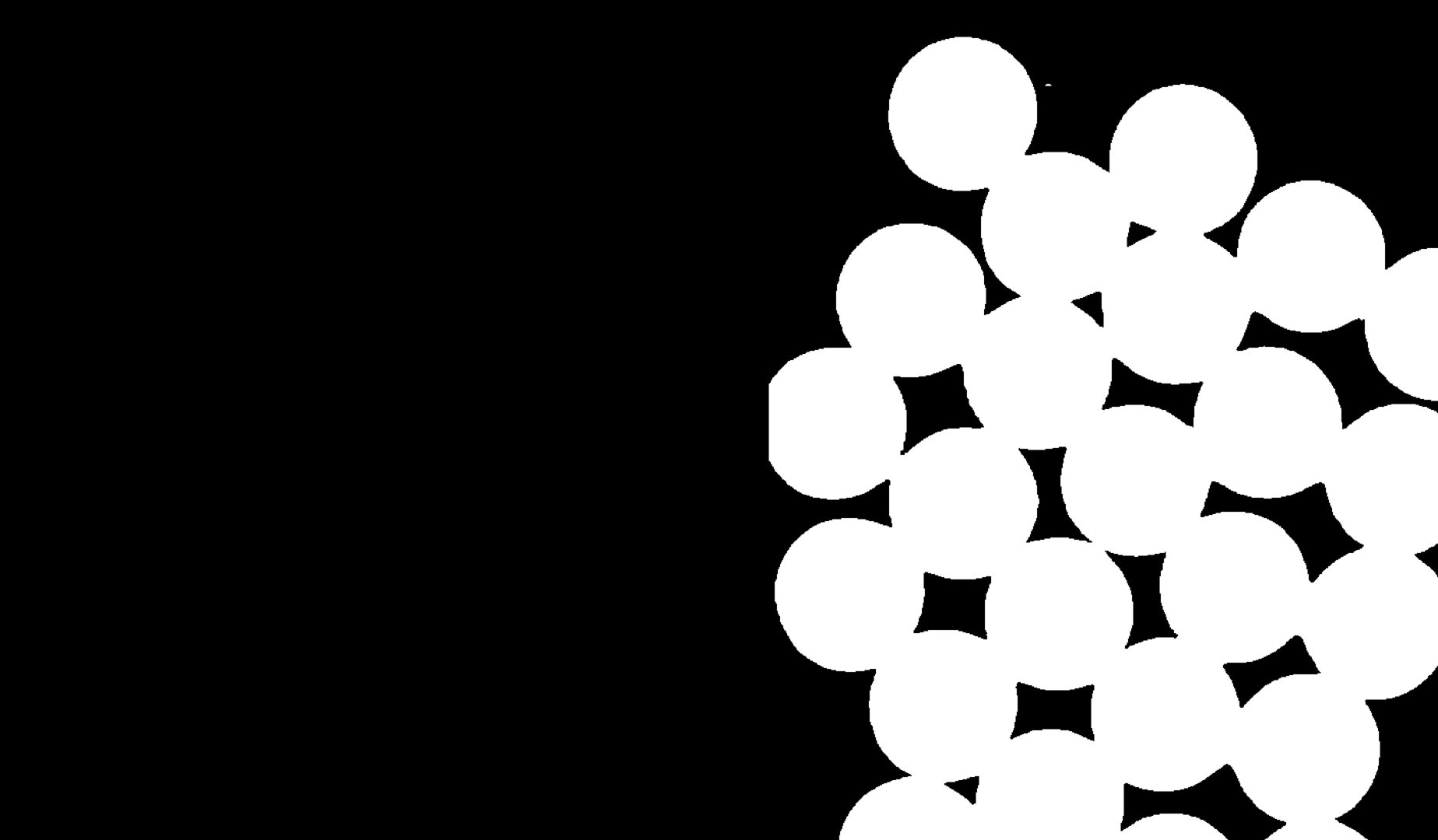
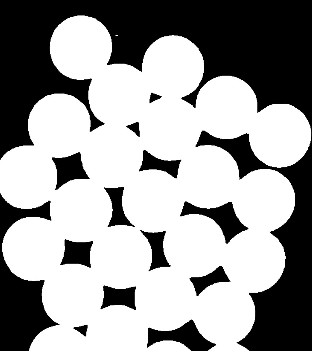
watershed
使用距离变换和分水岭来分割相互接触的物体
靠近对象中心的区域是前景,离对象远的区域是背景,不确定的区域是边界。
-
物体没有相互接触/只求前景 可用侵蚀消除了边界像素
-
到距离变换并应用适当的阈值 膨胀操作会将对象边界延伸到背景,确保background区域只有background
边界 = 能否确认是否是背景的区域 - 确定是前景的区域
1 | |

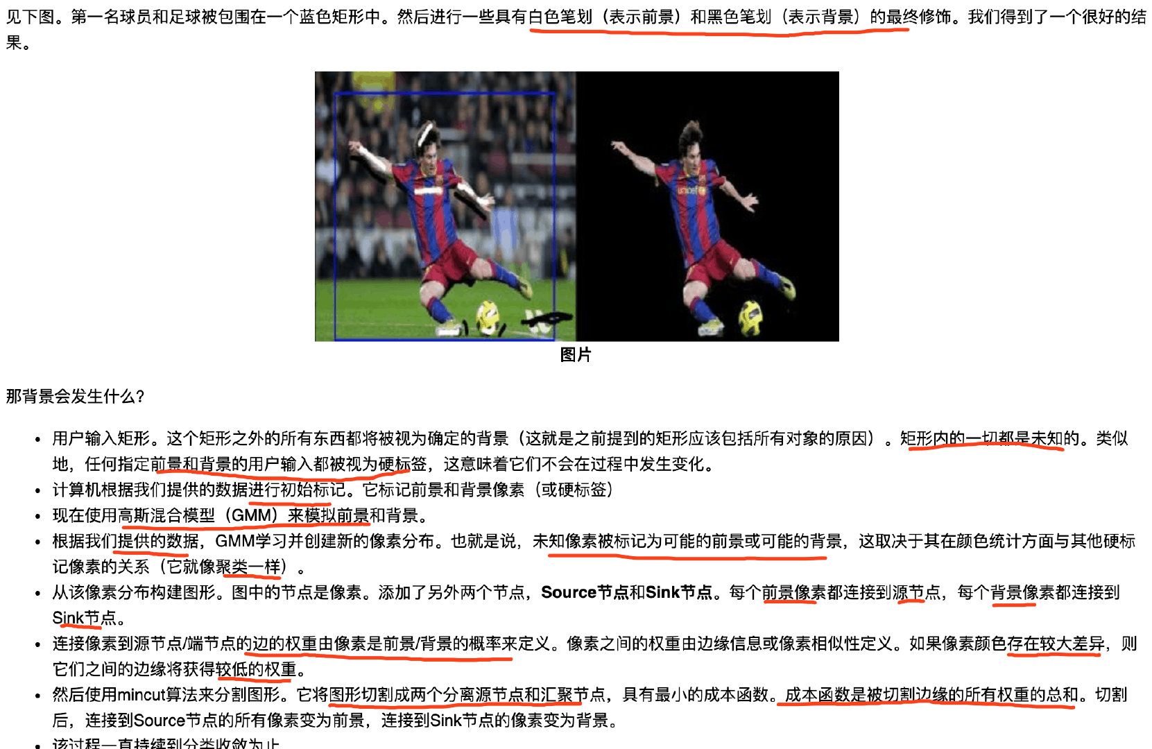
GrabCut
提取图像中的前景
- 用户在前景区域周围绘制一个矩形(前景区域应该完全在矩形内)
- 算法迭代地对其进行分段以获得最佳结果
某些情况下,分割将不会很好。某些前景区域标记为背景,用户需要做标记前景和后景
算法过程 就是监督半监督学习 根据颜色相似性 聚类分割
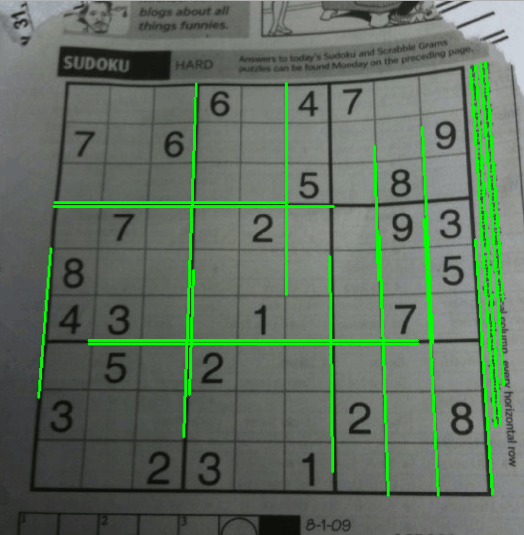
Hough
检测直线 霍夫变换
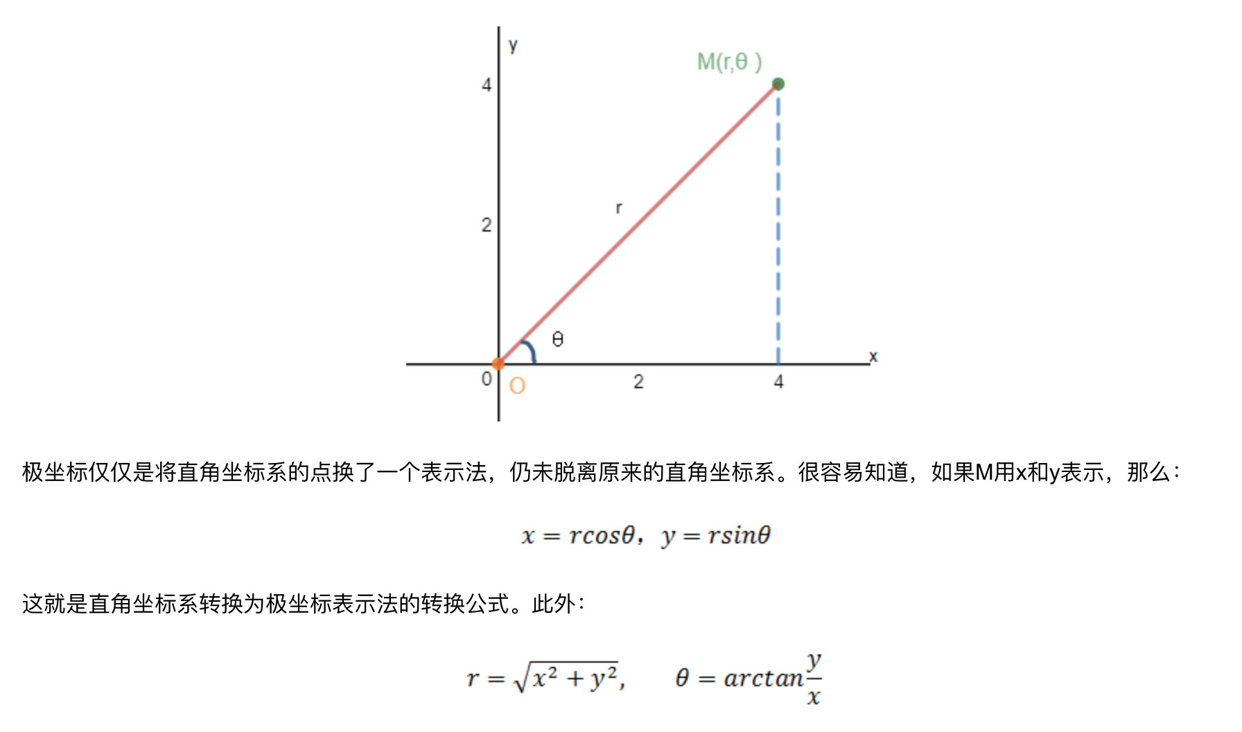
极坐标
1 | |
pyramid
有不同分辨率的相同图像
不同分辨率的图像就是图像金字塔 小分辨率的图像在顶部,大的在底部
低分辨率的图像由高分辨率的图像去除连续的行和列得到
1 | |
复杂例子 模糊边界
1 | |
Contour
轮廓
概念
what is contour
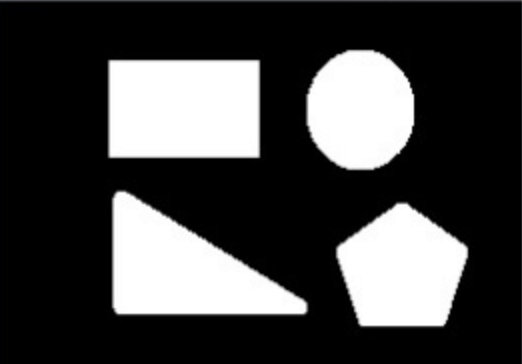
轮廓 是连接所有连续点(沿着边界)的曲线,具有相同的颜色或强度。轮廓是形状分析和物体检测和识别的有用工具。
从黑色背景中找到白色物体
hierarchy 层次结构
外部一个称为父项,将内部项称为子项,图像中的轮廓彼此之间存在某种关系。并且我们可以指定一个轮廓如何相互连接
每个轮廓都有自己的信息 [Next,Previous,First_Child,Parent] 没有为-1
- Next 表示同一层级的下一个轮廓
- Previous 表示同一层级的先前轮廓
- First_Child 表示其第一个子轮廓
- Parent 表示其父轮廓的索引
轮廓查找模式
- RETR_LIST 检索所有轮廓,但不创建任何父子关系 它们都属于同一层级 First_Child Parent = -1
- RETR_EXTERNAL 只返回最外边的轮廓,所有子轮廓会忽略
- RETR_CCOMP 所有轮廓并将它们排列为2级层次结构 对象的外部轮廓(即其边界)放置在层次结构-1中。对象内部的轮廓(如果有的话)放在层次结构-2中 如此类推
- RETR_TREE 检索所有轮廓并创建完整的族层次结构列表
1 | |
轮廓逼近法
轮廓中会存储所有边界上的(x,y)坐标。但是不一定需要全部存储
- cv.CHAIN_APPROX_NONE,则存储所有边界点
- cv.CHAIN_APPROX_SIMPLE 它删除所有冗余点并压缩轮廓,从而节省内存
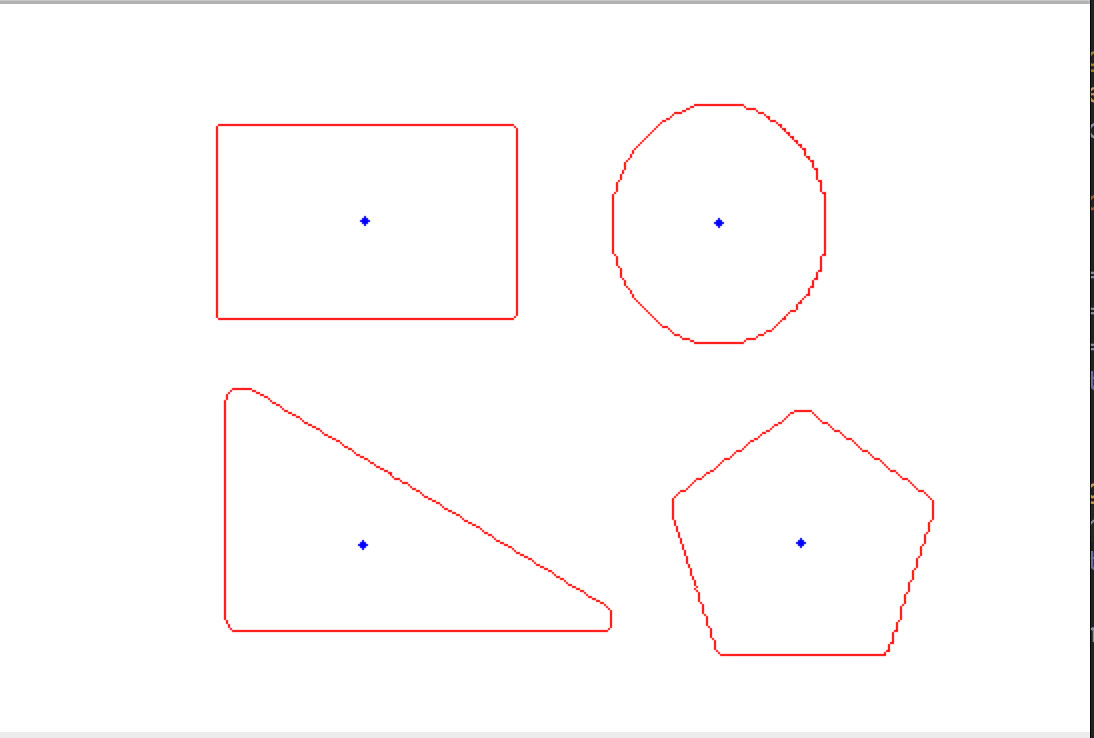
质心 面积 周长
1 | |
approx 轮廓近似
用更少点组成的轮廓
1 | |
Convex Hull
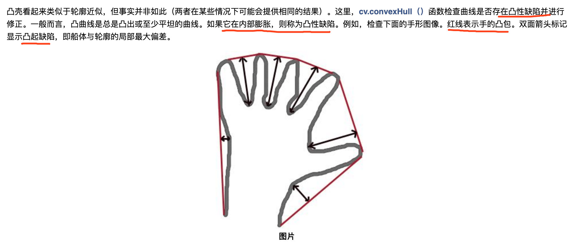
类似于轮廓近似
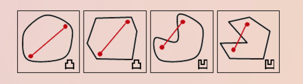
凸包: 在多维空间中有一群散佈各处的点 ,凸包 是包覆这群点的所有外壳当中, 表面积暨容积最小的一个外壳,而最小的外壳一定是凸的。
凸的定义: 图形内任意两点的连线不会经过图形外部
凸性缺陷:
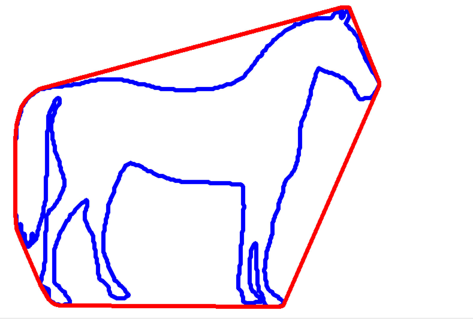
求凸包
1 | |
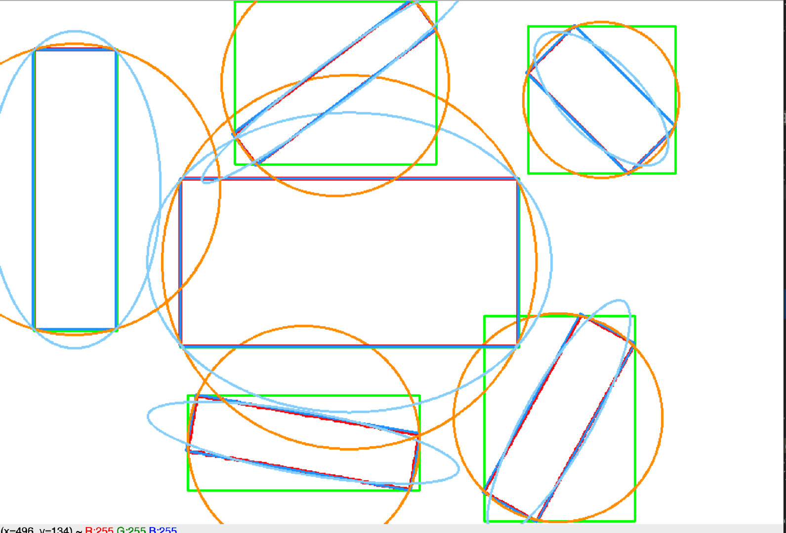
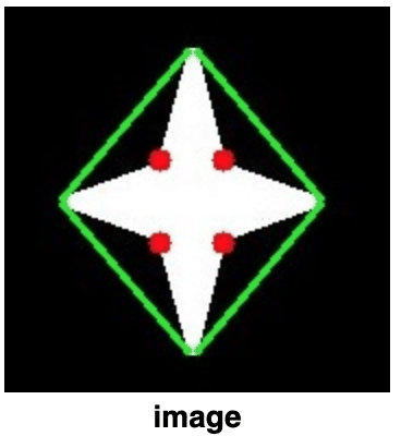
边界矩形 边界标注
Bounding Rectangle
1 | |
其他
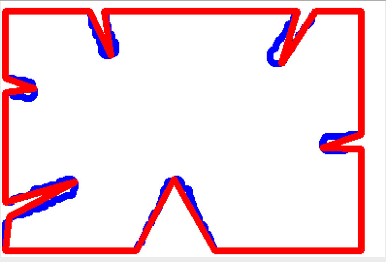
凸性缺陷
1 | |
点多边形距离
(50,50) 点与轮廓之间的最短距离 当点在轮廓外时返回负值,当点在内部时返回正值,如果点在轮廓上则返回零
1 | |
匹配形状
越相似越小 一样 =0.0
1 | |